Bayesian Triage Engine
A robust framework for objective veterinary triage.
What is a Bayesian Triage Engine?
It is a probabilistic inference system that, given observed inputs (symptoms, clinical signs, blood reports, and other lab results), computes two key outputs: the probability of each possible disease and the probability of organ dysfunction. The engine combines the prior disease prevalence, the likelihood of each symptom given a disease, and the patient's actual reported symptoms using Bayes' theorem. Through this calculation, it produces a posterior probability distribution over diseases and a separate probabilistic estimate for organ dysfunction – a quantitative foundation for clinical decision‑making.
1. Bayes' Theorem – Updating Beliefs with Evidence
At its core, Bayes' theorem formalises a simple intuition: your belief about a hypothesis should change when you see new evidence.
We begin with a prior probability – how common the disease is in the relevant population. Then we observe symptoms; each disease has a known likelihood (e.g., "if a patient has the flu, 90% chance of fever"). The engine multiplies the prior by these likelihoods for all reported symptoms, then normalises so that probabilities sum to 100%. The result is the posterior probability – your updated belief after seeing the evidence.
To make this practical, the engine adopts the "naive" assumption: symptoms are conditionally independent given the disease. This simplifies the calculation enormously (from a joint probability to a product of individual likelihoods). Although rarely perfectly true, naive Bayes works well for medical triage. However, multiplying many tiny probabilities risks numerical underflow – which is why we use the log‑sum‑exp trick (Section 3).
More complex dependencies between symptoms (beyond the naive assumption) can be handled using factor graphs and belief propagation – a general framework that still performs efficient probabilistic inference. We explore this next.
2. Factor Graphs & Belief Propagation – How Messages Flow
What is a Factor Graph?
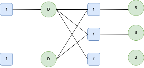
A factor graph breaks a probabilistic model into variable nodes (diseases or symptoms) and factor nodes (relationships between variables). Edges only connect variables to factors, which generalises the naive Bayes model and enables efficient computation.
Factor graph for two diseases (D₁, D₂) and three symptoms (S₁, S₂, S₃)
How Belief Propagation Works – Messages in Three Nodes
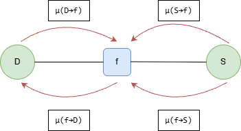 Figure: Message flow in both directions – D ⇄ F ⇄ S.
Belief propagation sends messages along every edge – think of them as notes carrying probability information. Each node passes its current belief to neighbours and receives updated beliefs in return. For example, an observed symptom's value flows back to the disease (pushing evidence forward), while a disease's prediction flows forward to a symptom (pulling predictions backward).
In a larger network, nodes exchange messages repeatedly until all agree on consistent probabilities – convergence. The final belief at each disease node is the diagnostic answer. If the graph contains loops, loopy belief propagation still works, requiring a few extra rounds.
Bottom line: Belief propagation turns a static factor graph into a two‑way conversation, reaching an agreement efficiently without recalculating everything from scratch.
3. Maintaining Numerical Stability – The Log‑Sum‑Exp Trick
Multiplying many probabilities quickly leads to underflow – computers round tiny numbers to zero. To avoid this, we work in log space, where multiplication becomes addition. But we then need to sum probabilities, which is tricky in log space.
The log‑sum‑exp trick solves this: subtract the largest log‑value from all terms, exponentiate, sum safely, take the logarithm, then add the largest value back. The largest exponential becomes exactly one, so no extremely large or tiny numbers appear.
By applying this trick, the diagnostic engine can handle hundreds of input features (symptoms, clinical signs, blood reports) without numerical errors – numerically bulletproof inference.
Bottom line: The trick lets us stay in log space to prevent underflow while still summing probabilities correctly – safe and stable.